Week 3 - Classification Problem, Logistic Regression and Gradient Descent. PartI
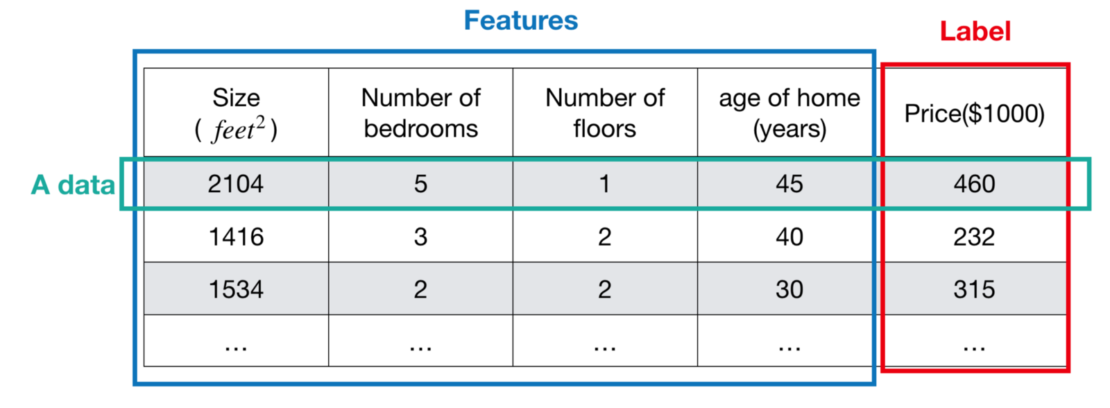
In week1 and week2, we introduced the Supervised Learning and Regression Problem. Today, we are going to discuss another problem in Supervised Learning — the Classification Problem. Before going into details, we should think about - what’s the difference between Regression Problem and Classification Problem? The answer is label type, the former is continuous number while the later is discrete number. In Regression Problem, a label is a continuous number (or real number). Taking Housing Price as example, according to the different combination of features, we can get the label (i.e. price) such as $460,000, $232,000, $315,000, etc. All of them are the actual value of the data.

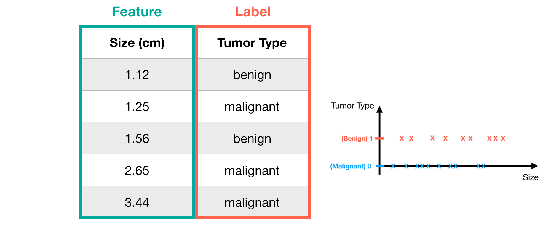
Whereas the label in Classification Problem represents ‘category’. Here we take breast cancer detection as an example. In breast cancer detection, what we concern most is the tumor type, that is, malignant or benign. For convenience’s sake, we simply labeled malignant and benign as 0 and 1 respectively. Note that the discrete number (0 and 1) means the label (tumor type) of the data.

Now we have the basic ideas of two problems. Let’s go into the details of Classification Problem!
Classification Problem
Hypothesis function
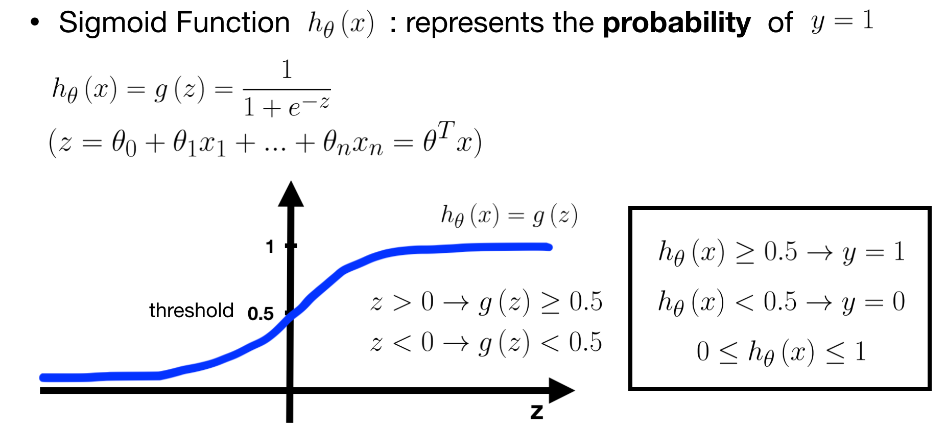
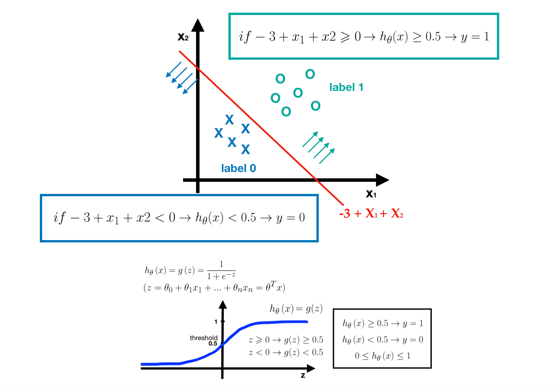
Since the label type is different from Regression Problem, we should use another hypothesis for solving Classification Problem. Here, we are going to introduce a popular one — Logistic Regression. Logistic Regression is also called a sigmoid function, which maps real numbers into probabilities, range in [0, 1]. Hence, the value of sigmoid function means how certain the data belongs to a category. The formula is defined as the following picture.
- Note that y represents the label, y=1 is the goal label and y=0 is the other label, and in sigmoid function, we always concern about the goal label.
- In most cases, we take 0.5 as the threshold of probability. If h(x)≥0.5, we predict the data belongs to label 1, while h(x)<0.5, we predict the data belongs to label 0.


In order to understand this concept more easily and clearly, let’s visualize the example and explain it step by step.
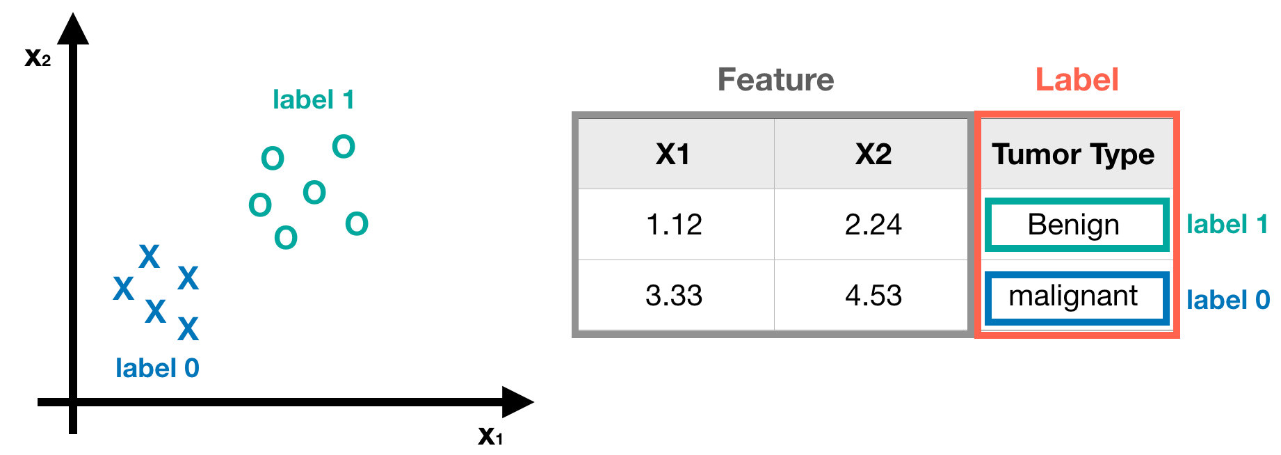
- Preparing Dataset - suppose we have a breast detection dataset, each one has two features and one label.

- Getting Parameters - after learning process, we get a nice model, that is, we get the parameters of logistic regression. Here, we assume they are -3, 1 and 1.

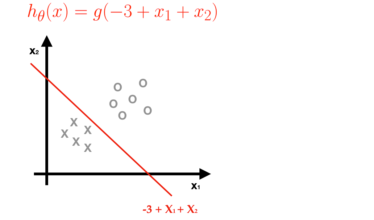
- Predicting Labels — according to the sigmoid function with learned parameters.
- If the -3+x1+x2≥0, it means h(x)≥0.5, then we predict this tumor is benign (label 1).
- If not, then we predict this tumor is malignant (label 0)

Understanding the concept of probability in logistic regression
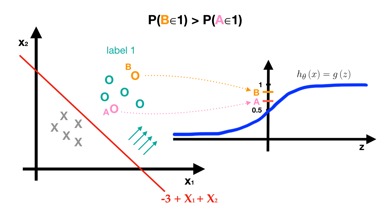
In the following picture, although the label of point A and point B are both 1, their probabilities are different, and P(B∈1)>P(A∈1). When a point is farther away from the redline, this label is more determinable. Whereas when a point is right on the redline, the predictor can’t surely determine which label the point shall belong to since the probabilities are the same, P(a∈label0)=P(a∈label1)=0.5. That’s quite intuition.

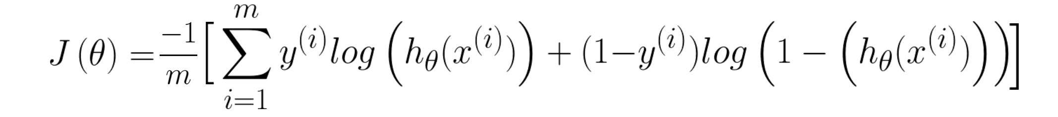
Cost Function
After learning process, we get the predictor - the logistic regression with learned parameters. To decide and improve the quality of the predictor, we need to define the Cost Function which measures the error that the hypothesis made and to minimize it.

Gradient Descend
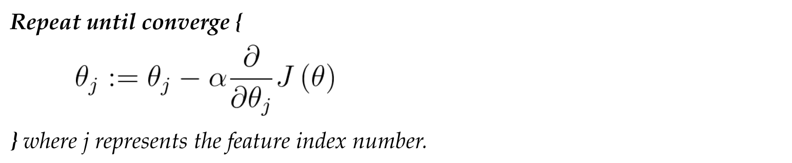
We can minimize the cost function by using gradient descent, the detail we discussed in previous note, please check here. In logistic regression, the gradient descent looks identical to linear regression.

Multi-class classification
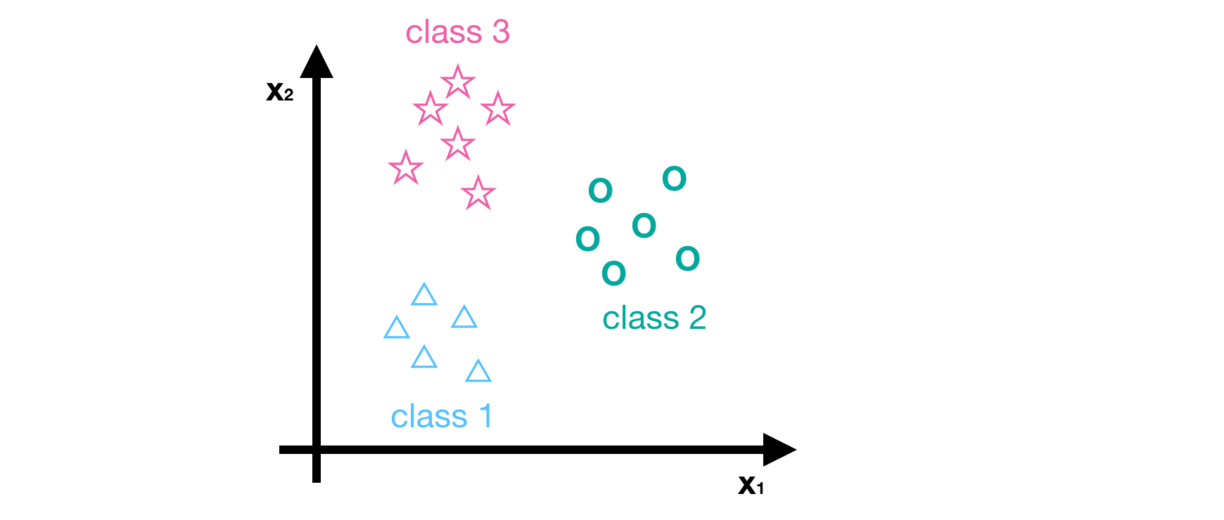
So far, we have only discussed the binary classification problem but we often meet the multi-class classification problem in reality, i.e. more than two labels. Here, we introduce a common method based on logistic regression, called one-vs-all or one-vs-rest. The core idea of one-vs-all method is to classify the dataset into positive class and negative class (i.e. goal class and the other classes) at each time, and then to get the probability of being the positive class. After calculating the probabilities of being all positive classes, we choose the maximum one as the predictor’s result. For example, suppose we have a dataset with three classes.
- Class1 (△)
- Class2 (◯)
- Class3 (☆)

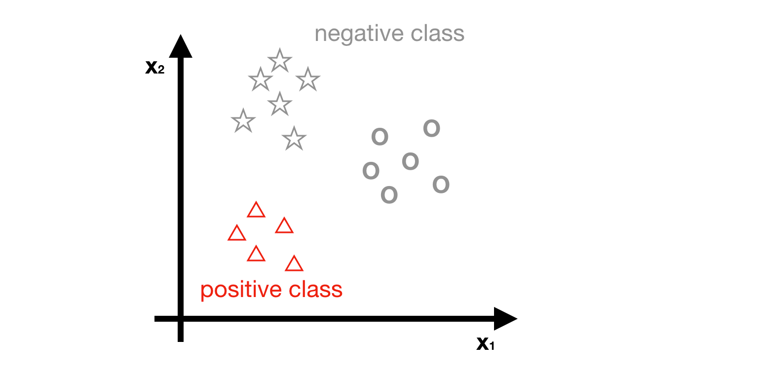
- Step1 - Choosing the class1 as positive class, and the other classes are negative class.

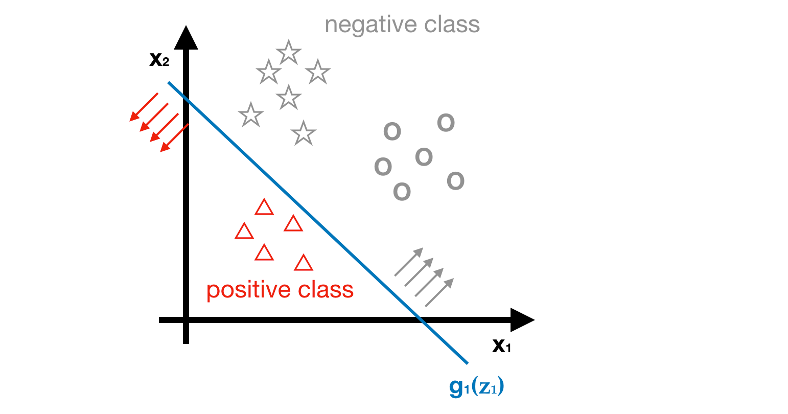
- Step2 - Suppose we get a predictor g1(z1) after learning process, we use this predictor to estimate the probability of being class1 (△)

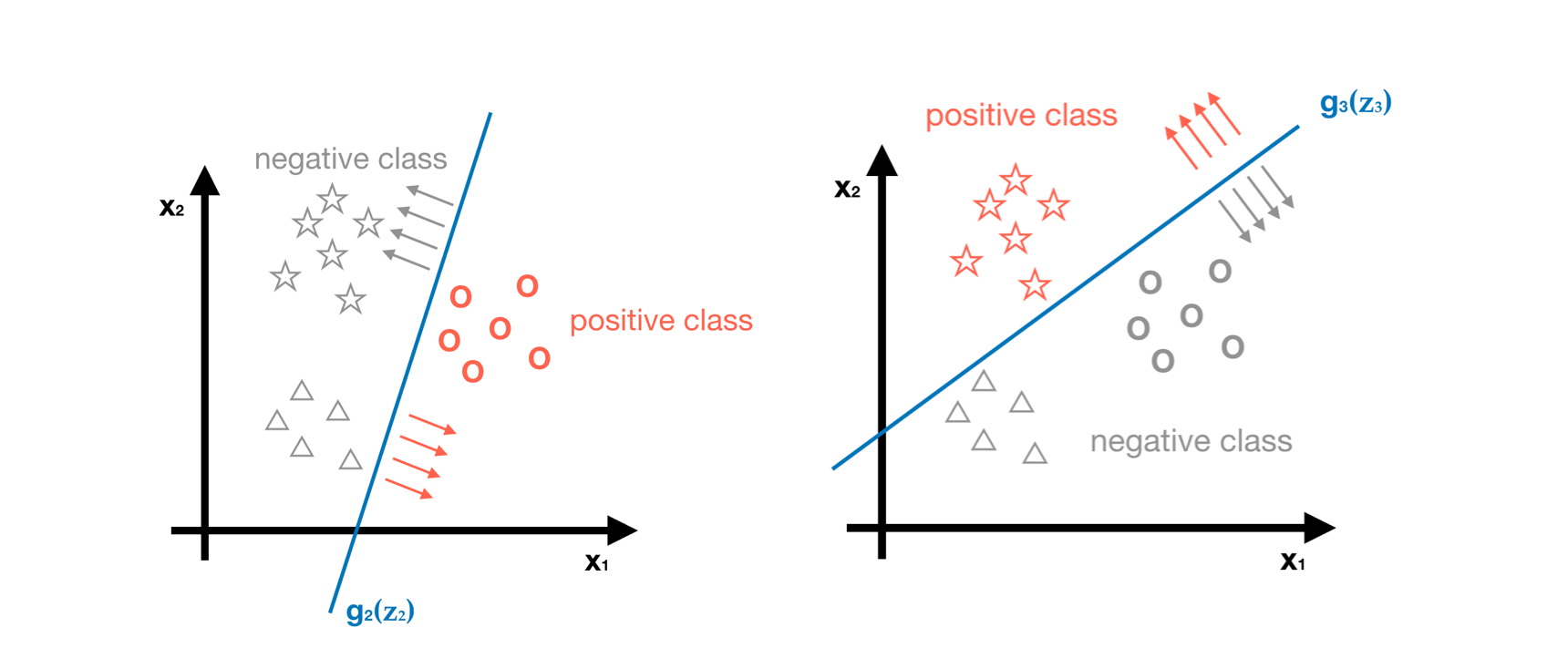
- Step3 - Repeat step1 and step2, but set a different positive class. Finally, we can get g2(z2) and g3(z3), as shown in the following picture. We use predictor g2 and g3 to estimate the probability of being class2 (◯) and class3 (☆) respectively.

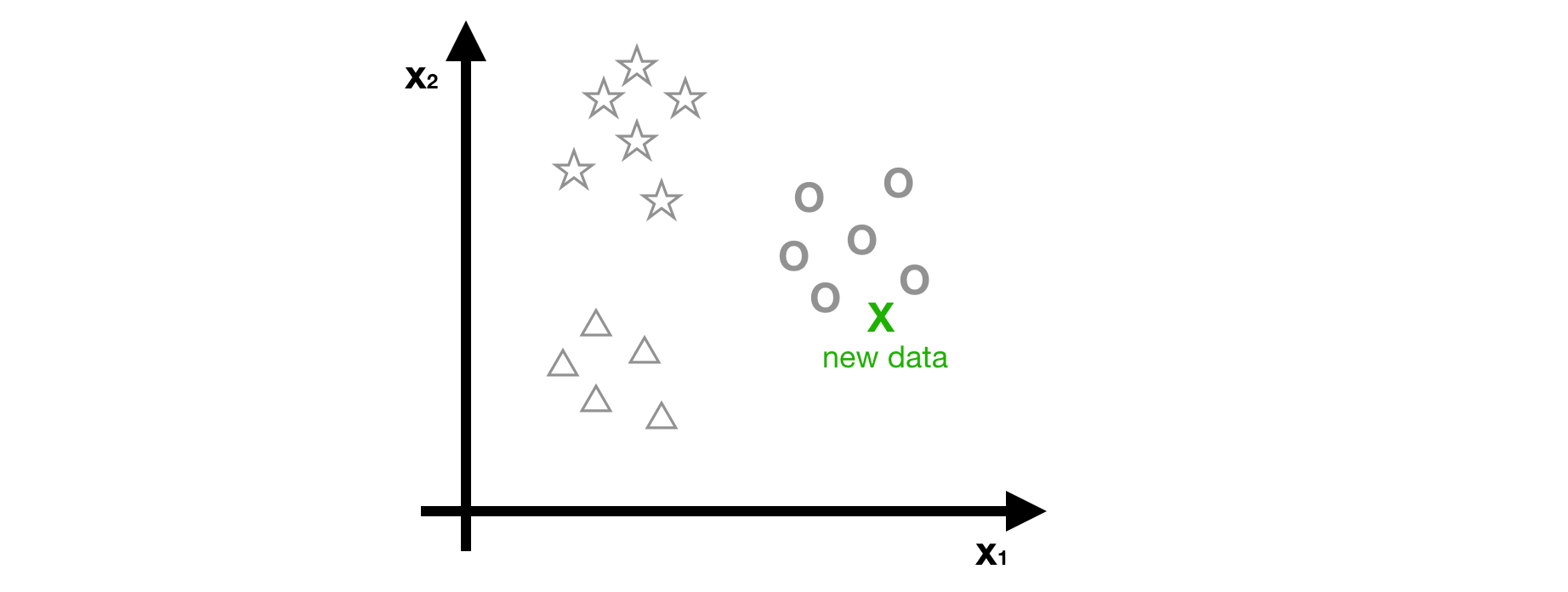
- Step4 - Predicting the class of new data by using three predictors, g1, g2 and g3.


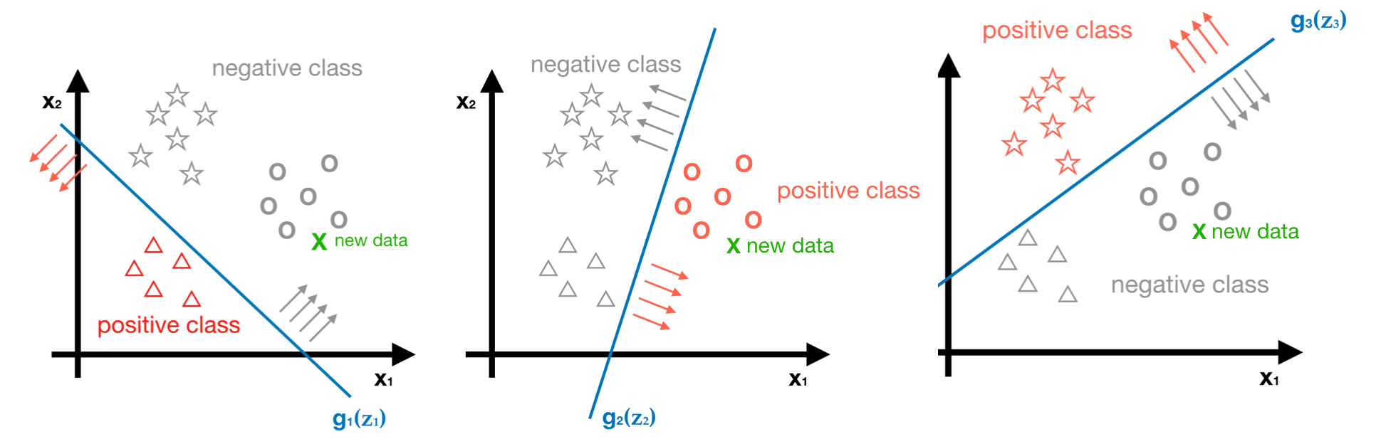
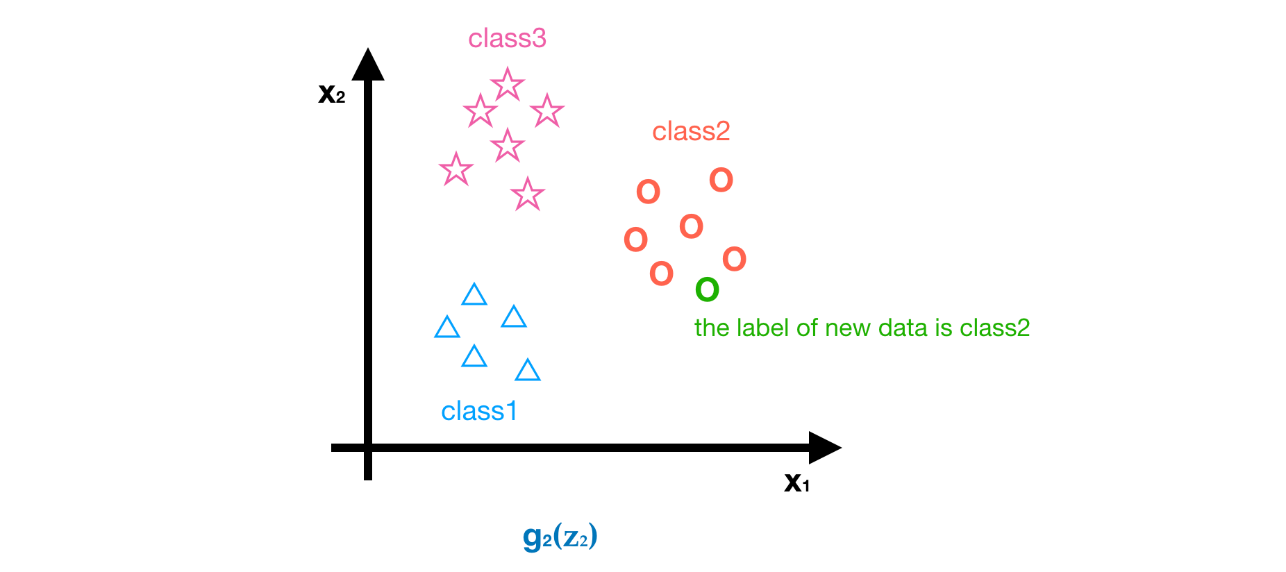
As you can see, the probabilities we get for the new data are g1<0.5, g2>0.5 and g3<0.5. The maxima is g2>0.5, Hence, we can conclude the predict label of this new data is class2 (◯).

If you want to do a project relate to classification problem, here is a reference for novices. Next part, we will be talking about two important concepts - Overfitting and Regularization.