Week 2 - ML(Coursera) - Multivariate Linear Regression, MSE, Gradient Descent and Normal Equation.
In Week1, we introduced the single variable linear regression. In this note, we will provide a concept of multivariate linear regression (i.e. multiple variables linear regression). There are three parts in this note,
- Part I - We will talk about multivariate linear regression and its cost function, Mean Square Error.
- Part II - How to minimize the cost function by using the Gradient Descent Algorithm, and provide a few skills to improve its performance.
- Part III - Introducing the Normal Equation Method, another way to solve multivariate linear regression.
PART I - Multivariate Linear Regression
Linear Regression with multiple features
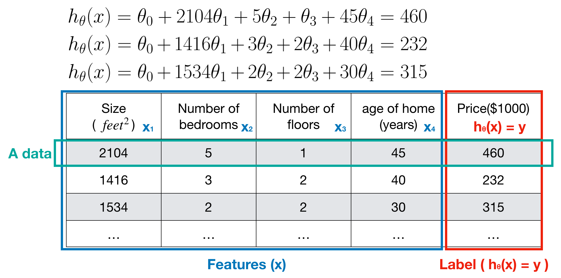
If we have a continuous labeled data with more than one feature, we can use the multivariate linear regression to make a machine learning model. The label is the answer to a data and the value is continuous (i.e. real numbers). With below housing price example, the label is price and the features are size, number of bedrooms, number of floors and age.


Note that there is only one true model for the data. Unfortunately, we don’t know what the true model is. And in order to find the true one, we make a hypothesis, tuning it until we can check if it is close enough to the true model or it is a wrong one (according to the criterion such as accuracy, precision, F1 score etc.). If the hypothesis is wrong, then make another one and tune it. When choosing a model, be utmost care about making the hypothesis. Per above housing price example, suppose the true model for the data is linear, then we can try to use linear regression and its hypothesis function.
Hypothesis function
In Multivariate Linear Regression, the hypothesis function with multiple variables x and parameters θ is denoted below.

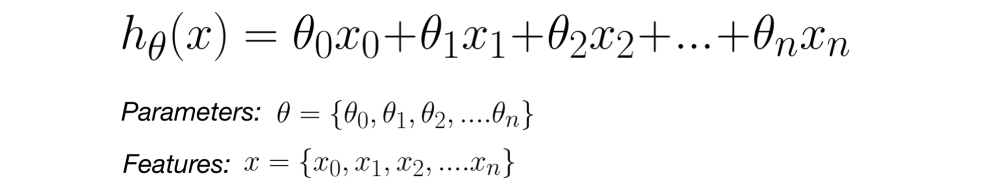
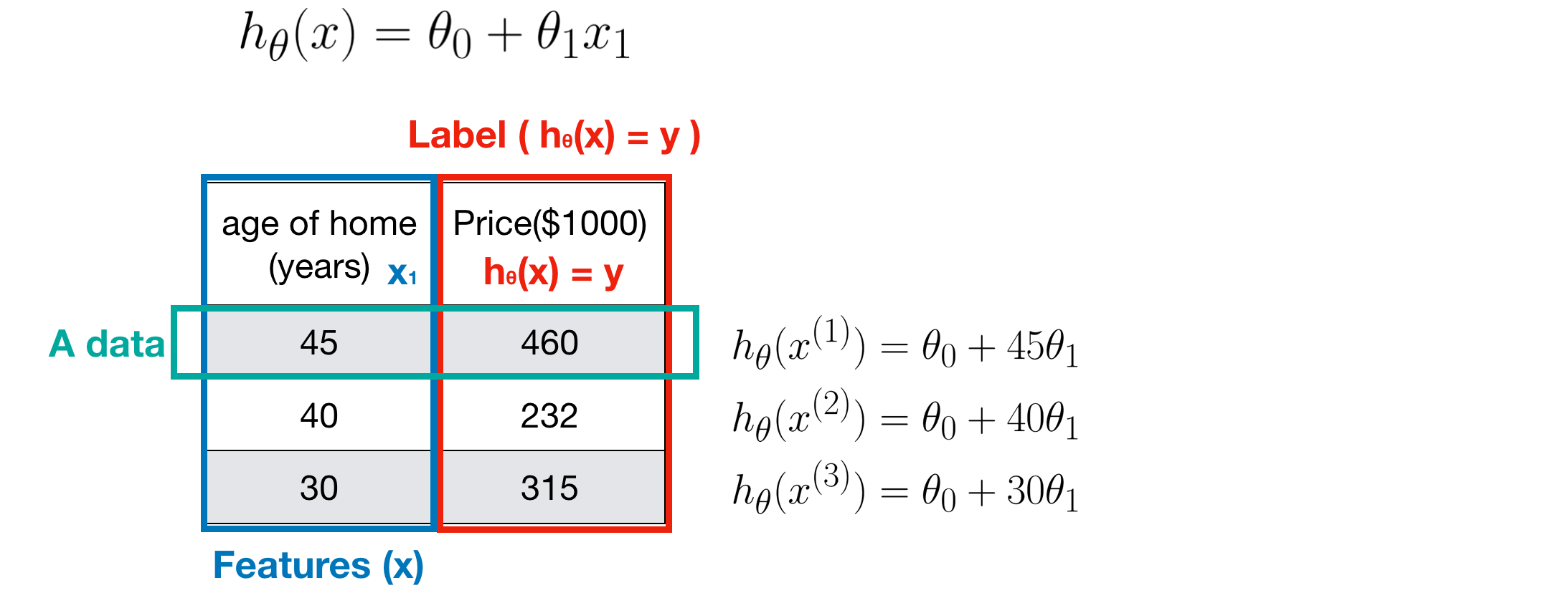
The following example shows that how to use the hypothesis function.

When tuning the hypothesis, our model learns parameters θ which makes hypothesis function h(x) a ‘good’ predictor. A Good predictor means the hypothesis is closed enough to the true model. The closer, the better. But how do we know the hypothesis h(x) is good enough or not? The answer is using a cost function, which we defined to measure the error that the hypothesis made.
Cost Function
The accuracy of Hypothesis Function h(x) can be measured by using Cost Function.
In Regression Problem, the most popular cost function is Mean Error Square(MSE). The formulation is defined as below.

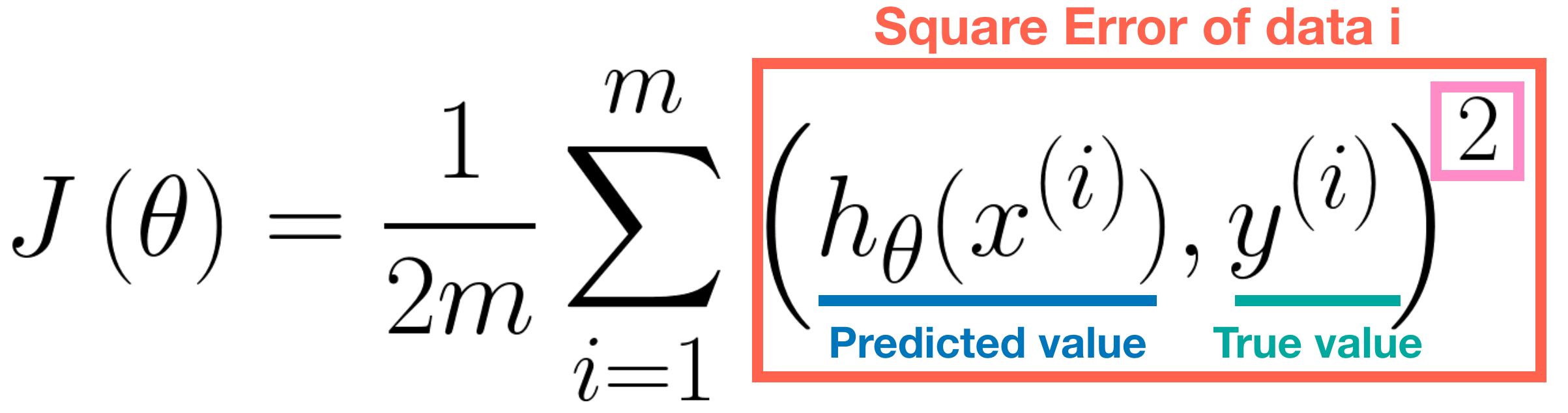
Note that the square (see above pink rectangle) is necessary since an error value is always positive. Moreover, the square error function is differentiable, thus we can apply the Gradient Descent Algorithm to it. Essentially, the cost function J(θ) is the sum of the square error of each data. The larger the error, the worser the performance of the hypothesis. Therefore, we want to minimize the error, that is, minimize the J(θ).
PART II - Gradient Descent Algorithm
Gradient Descent Algorithm is a common method for minimizing cost function. Once the minimum error is found, the model learns the best parameters θ in the meanwhile. Thus, we probably find the good predictor, a hypothesis function with the best parameters θ that makes the minimum error. Note that we use the word ‘probably’ here, since the hypothesis with the best parameters θ may suffer from the problem, the so called ‘overfitting’. We will discuss it in other section.
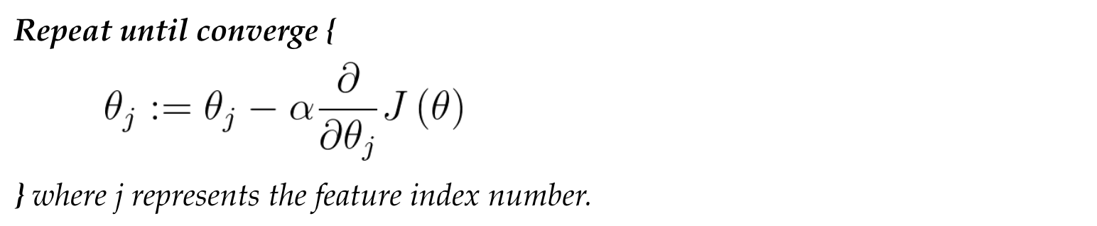
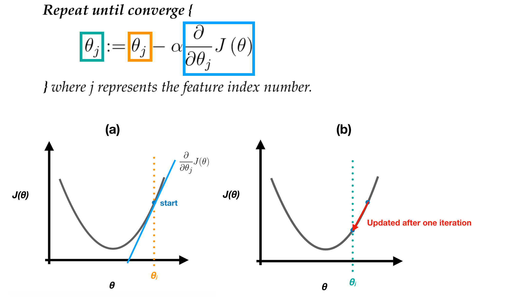
Pseudocode
At each iteration, the parameters θ need to be updated simultaneously.

In order to get a better understanding of the Gradient Descent Algorithm easily, we visualized the steps in following figure. In figure (a), the starting point is at orange (θj, J(θj)). Calculate its partial differentiation, then multiplied it by a learning rate α and the updated result is at green (θj, J(θj)), as figure (b) shows.

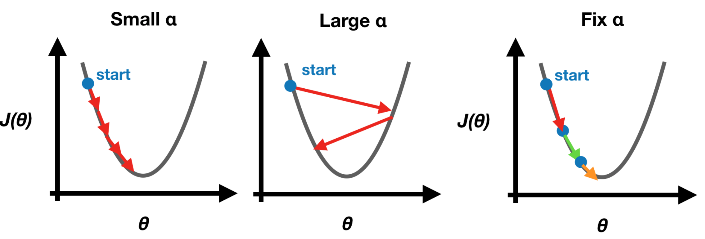
Learning rate α
We use learning rate α to control how much we update at one iteration. If α is too small, it makes the gradient descent update too slow, whereas the update may overshoot the minimum and won’t converge. Note that we set a fixed learning rate α in the beginning since the gradient descent will update slowly and automatically until it reaches the minimum. Hence, there is no need to change the learning rate α at each iteration by ourselves.

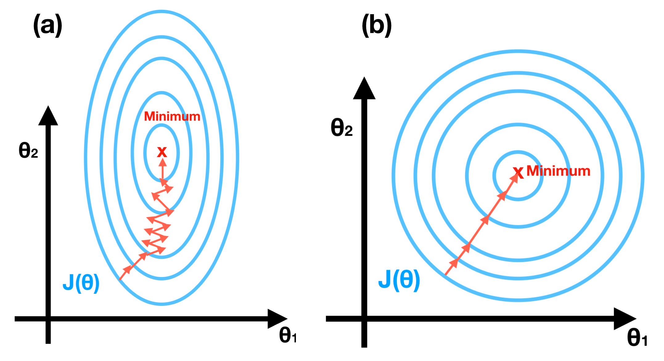
Make Gradient Descent Well
In this segment, we provide two skills, Feature Scaling and Learning Rate, to ensure the gradient descent will work well. Feature Scaling, also called normalized features. With different range of each feature, the contours may be extremely skinny, which will make Gradient Descent suffer from extremely slow, see Figure(a). After feature scaling, the outcome shows in Figure(b). It’s worth making sure that the features are on a similar scale and roughly within the range [-1, 1].

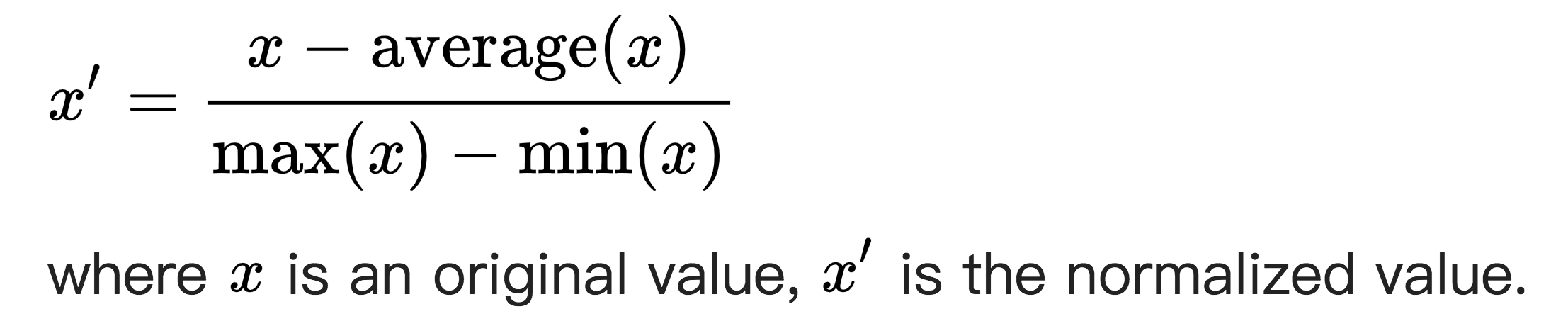
One way to scale features is Mean Normalization, the formula is

Learning Rate α - How to choose the value of α? According to the suggestion from Adjunct Professor Ng, is to try …, 0.001, 0.003, …, 0.01, 0.03, …, 0.1, 0.3, …, 1, …
PART III - Normal Equation Method
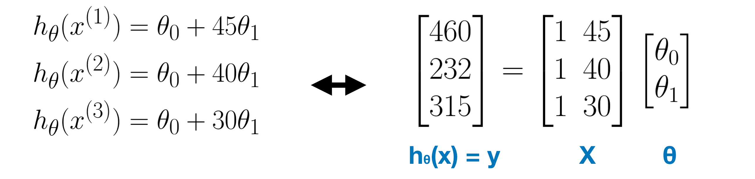
Normal Equation Method is very useful when solving the Linear Regression Problem. Take a simple example - Linear regression with single variable. In the following figure, there are three linear equations as we have three data.

In linear Algebra, linear systems can be represented as the matrix equations.

If you are familiar with the concept of Pseudo Inverse in Linear Algebra, the parameters θ can be obtained by this formula:


In Multivariate Linear Regression, the formula is the same as above. But, what if the Normal Equation is non-invertible? Then consider deleting redundant features or using the regularization. To sum up, the advantages in using Normal Equation are
- No need to choose learning rate α
- No need to iterate
- Feature scaling is not necessary
Note that if the number of features is very large, the Normal Equation works extremely slow, while the Gradient Descent Algorithm still works well.
Next week, we will discuss Classification Problem and one of the popular hypothesis - Logistic Regression. If you are interested, see here.
Thanks for reading, and if you like it, please give me a 👏. Any feedbacks, thoughts, comments, suggestions, or questions are welcomed!