Week 3 (Part II) - Overfitting and Regularization
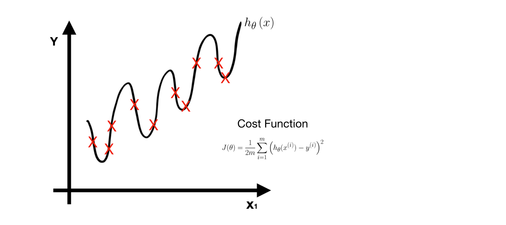
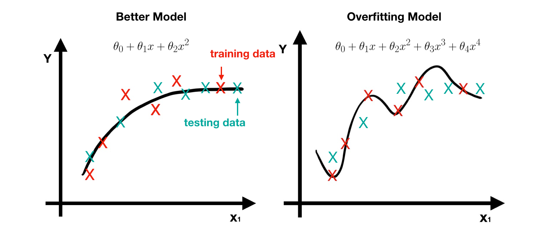
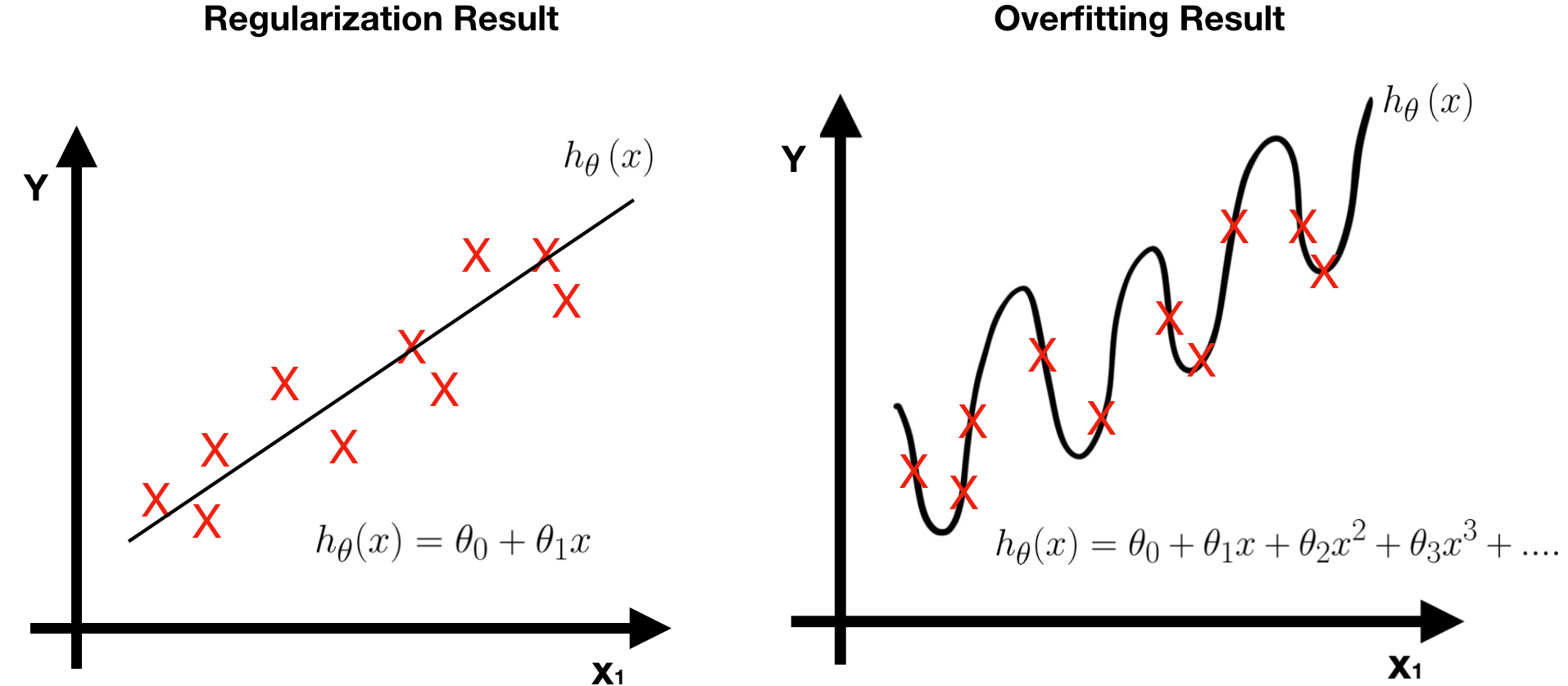
After learning process, we get a good model. If we apply it to certain problems, we may or may not get good performance. That is the issue we are going to discuss today — How come the performance of a good model is terrible? Let’s think it first— what is a good model? In the previous note, the definition of a ‘good’ model is the one with least training error. First, define a hypothesis function H **(i.e. model). Second, define a Cost Function **J(θ) for error measuring. Third, learn parameters of **H by minimizing **J(θ). In the end, we can get a learned model with least training error. In the extreme case, this ‘good’ model has zero training error and fits training data perfectly, that is, the predict label of all training data is equal to their corresponding truth label. Taking linear regression as example, the model fits all training data (red points) perfectly.

However, when new data (green point) comes in, this model has terrible performance with huge prediction error.

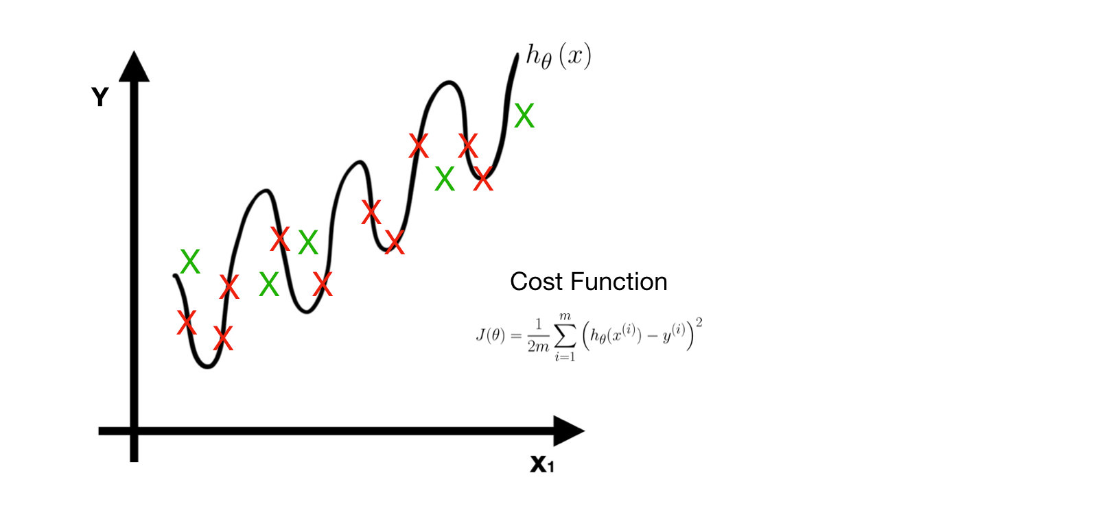
The problem here is called Overfitting. A truly good model must have both little training error and little prediction error.
Overfitting
The learned model works well for training data but terrible for testing data (unknown data). In other words, the model has little training error but has huge perdition error.
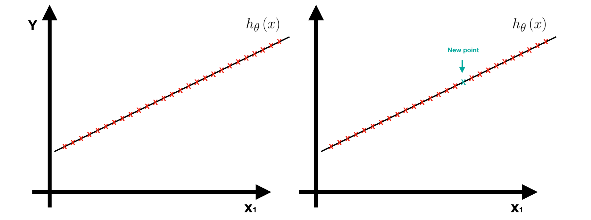
If we have a whole dataset that captured all possibilities of the problem, we don’t need to worry about overfitting. When new data comes in, it shall fall into one possibility, hence, the model can predict it perfectly. For example, suppose we have a training dataset that captures all points on the line and also get a perfect model h(x) with zero training error. Whenever new data comes in, it shall be one of the points, hence, the prediction error must be zero. In this special case, overfitting is not a problem.

Unfortunately, the training data we get in reality is normally a small part of the whole dataset. Therefore, even if the model fits these training data perfectly, this is still not a good model and overfitting must occur. When overfitting occurs, we get an over complex model with too many features. One way to avoid it is to apply Regularization and then we can get a better model with proper features.
Regularization
It’s a technique applied to Cost Function J(θ) in order to avoid Overfitting.
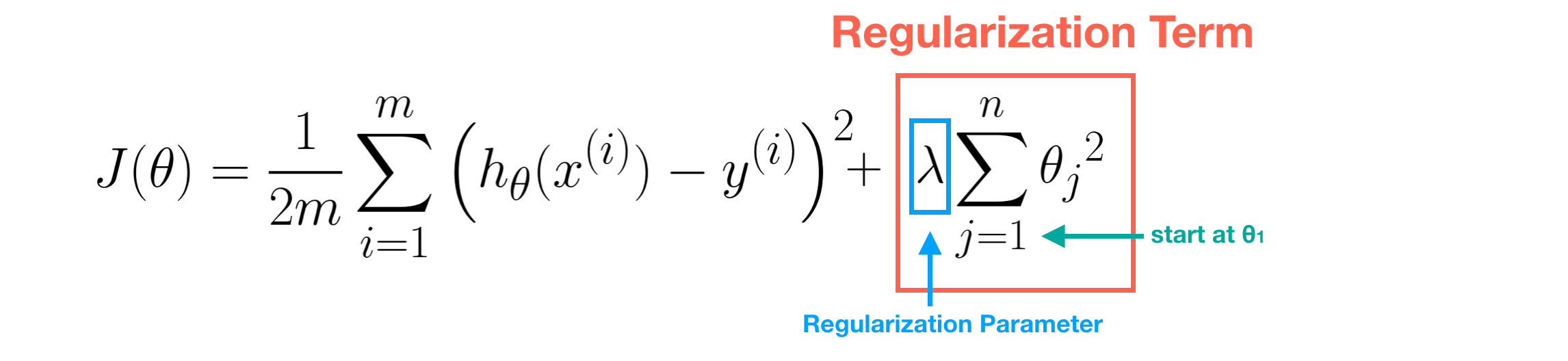
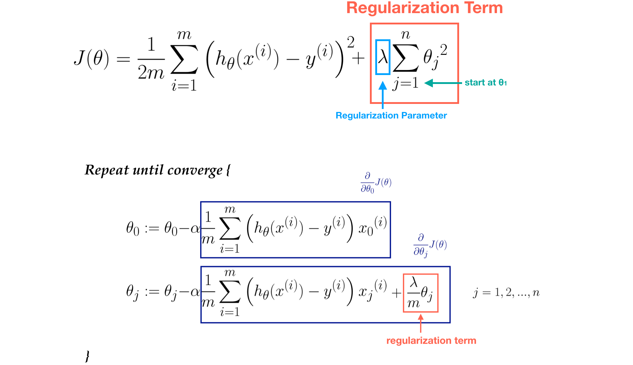
The core idea in Regularization is to keep more important features and ignore unimportant ones. The importance of feature is measured by the value of its parameter θj. In linear regression, we modify its cost function by adding regularization term. The value of θj is controlled by **regularization parameter **λ. **Note that **m is the number of data and n is the number of features(parameters.

For instance, if we want to get a better model instead of the overfitting one. Obviously, we don’t need features X³ and X⁴ since they are unimportant. The procedure describes below.

First, we modify the Cost Function J(θ) by adding regularization. Second, apply gradient descent in order to minimize **J(θ) and get the values of θ3 and θ4. After the minimize procedure, the values of θ3 and **θ4 must be near to zero if λ=1000.

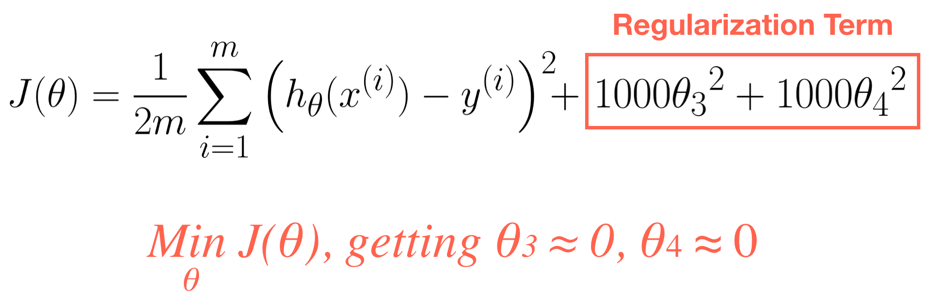
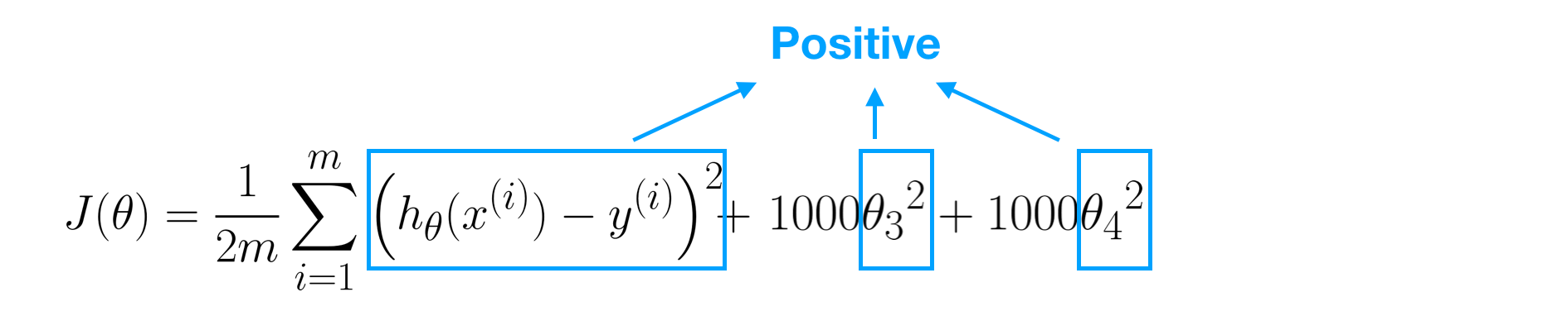
Remember, the value of J(θ) represents training error and this value must be positive (≥0). The parameter λ=1000 has significant effect on J(θ), therefore, θ3 and θ4 must be near to zero (e.g 0.000001) so as to eliminate error value.

Regularization Parameter λ
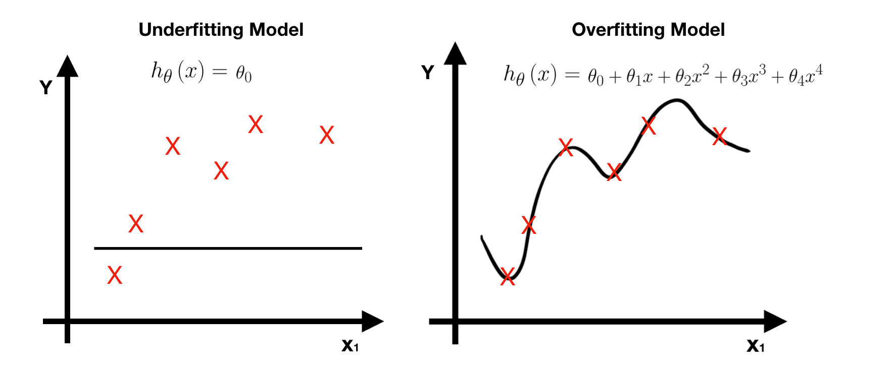
- If λ is too large, then all the values of θ may be near to zero and this may cause Underfitting. In other words, this model has both large training error and large prediction error. (Note that the regularization term starts from θ1)
- If λ is zero or too small, its effect on parameters θ is little. This may cause Overfitting.

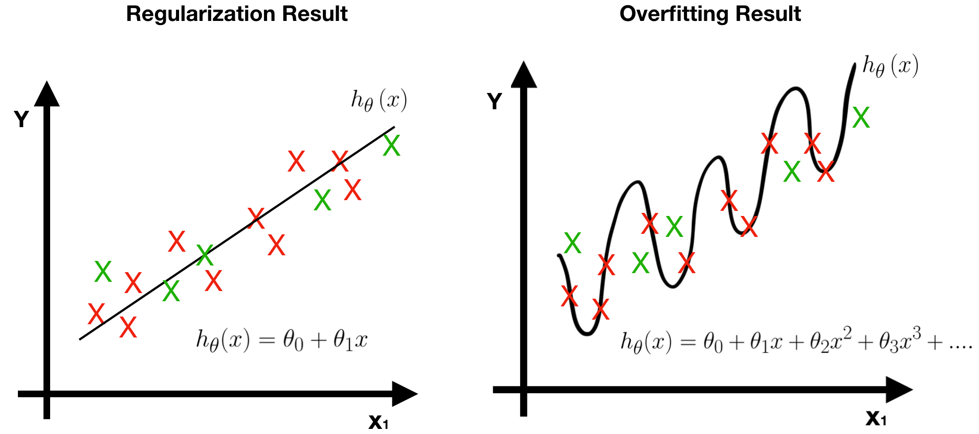
To sum up, there are two advantages of using regularization.
- The prediction error of the regularized model is lesser, that is, it works well in testing data (green points).
- The regularization model is simpler since it has less features (parameters).


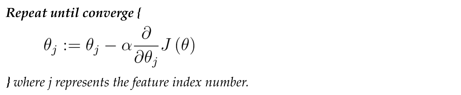
So far, we have discussed the concept of regularization. Next, we will show how to minimize regularized cost function by using gradient descent.
Recall: Gradient Descent

Regularized linear regression
If you are not familiar with linear regression, please see here.

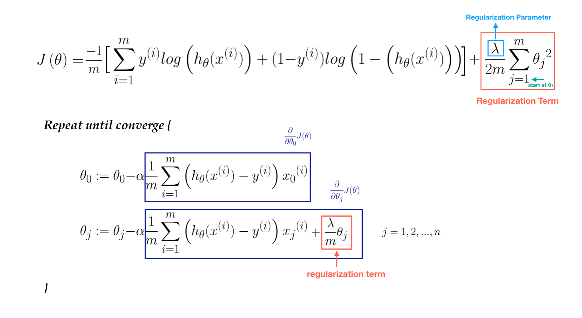
Regularized logistic regression
If you are not familiar with logistic regression, please see here.

Next week, we are going to introduce a popular topic — Neural Network, numerous Neural Network Architectures have been developed and applied to applications widely.